A practical Introduction to Vectors

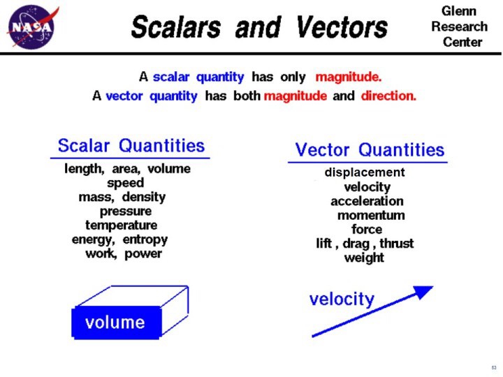
The mathematical concept of a “vector” is ubiquitous in the realms of physics, engineering and applied mathematics. Typically, the concept is first introduced (usually in a first semester physics course or perhaps a trigonometry or calculus course) as a quantity with both a magnitude and a direction, and is usually represented as a line segment with an arrow at the end of it (like a ray).

Often, these introductory treatments will distinguish what a vector is by contrasting it to what a scalar is. A scalar is just a quantity (albeit possibly with some units of measurement), such as length, weight, mass, speed, an amount of money, or a frequency. On the other hand, examples of vectors would be things like velocity, acceleration, force, momentum, and position (relative to some set of coordinates). In other words, they have a direction as well as a magnitude.

Although vectors can in principle be adapted to any coordinate system, for the sake of simplicity, we will presuppose a Cartesian coordinate system in either 1, 2, or 3 dimensions. In this representation, we’ll have a horizontal x axis and a vertical y axis for 2D, and for 3D we’ll have the y axis horizontal, the z axis vertical, and the x axis coming out of the page at the reader. This is just a matter of historical convention. Occasionally one might see the z axis being used as the one coming out of the page, but most of my pictorial examples involved the former and not the latter. This is a type of coordinate system with what’s called an “orthonormal” basis. I’ll cover the concept of a basis in a later post, but in practical terms, orthonormal just means that the coordinate axes are perpendicular to one another. Any points or vectors in the space are constructed by adding linear combinations of  unit vectors (magnitude equal to 1) in the x, y and z directions.

A vector can be represented by a letter with a little arrow on top of it. but since it’s a PITA to write them that way in this format, I’ll just use capital letters to name vectors for now. Suppose we have a vector, A. There are a number of common notational conventions for representing it.

A = [a1, a2, a3],

or

Image source

where the i, j and k with the little hats each represent a unit vector (a vector of unit length) in one of the component directions (x, y, and z respectively in this case), and the a1, a2 and a3, (or A_x, A_y and A_z) symbols represent the “components” of the vector in the x, y and z directions respectively. I will use the A = [a1, a2, a3] format for convenience.

So, for example, supposing you were traveling at 10 m/s in the x-direction. Then your velocity vector v = [10, 0, 0] m/s, since you’re not moving in the y or z directions at all.

Vectors can be added and subtracted just like scalar quantities. There are two commonly taught ways of doing this. They are the component approach and the geometric approach respectively. With the component approach, as the name implies, the process is to add or subtract each component of the vector.

For example, if you had a vector, A = [a1, a2, a3], and another vector, B = [b1, b2, b3].

Then A + B = [a1 + b1, a2 + b2, a3 + b3].

Similarly, A – B = [a1 – b1, a2 – b2, a3 – b3].

Let’s try a more concrete example. Supposing your positive x component corresponded to East, your positive y component corresponded to North, and your positive z component corresponded to up in the air. Supposing you had two cars driving in an open field. Car A has a velocity v_a = [40, 30, 0] km/hr, (that’s diagonal motion of 40 km/hr east and 30 km north) relative to an observer on the ground, and car B is moving at a velocity v_b = [0, -40, 0] km/hr.

If you wanted to know A’s velocity from the perspective of B, then you’d subtract the velocity of B from the velocity of A.

v_a – v_b = [ 40 – 0, 30 – (-40), 0 – 0] km/hr = [40, 70, 0].

The following Khan Academy video explains some more examples of this.

As for the geometric approach to vector addition, supposing you had two vectors u and v, and you wanted to draw their sum: u + v. The procedure would be to place the tail of v at the head of the u, and then draw a new vector from the tail of u to the head of v. This new vector is their sum: u + v. Here’s an illustration of this:

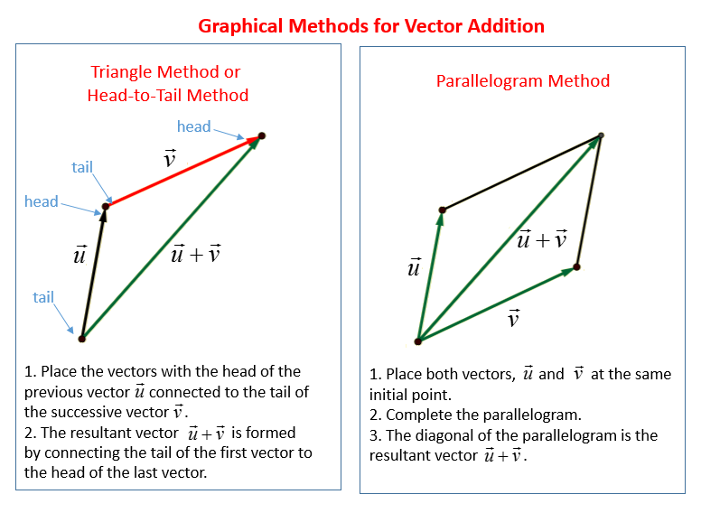
Geometric Approach to Vector Addition (image credit)

The same approach also works with vector subtraction. The only difference is that the arrow of the subtracted vector will point in the direction opposite to its usual direction.Here I’ve used examples of only two vectors, but both of these methods can easily be generalized to multiple vectors.

Something that is typically not mentioned in such introduction (mostly for the sake of expediency), is the fact that this definition of a vector is really only a special case of a much broader-reaching concept rife with many other special cases, each comprising their own unique attributes and applications. Later on, it is customary for the student to learn a more generalized concept of vector “spaces,” whereby a vector space is defined by a list of rules by which the elements of a space must abide in order to qualify as a vector space. This is traditionally taught in a first course on linear algebra, along with concepts such as “rank,” “dimension,” “linear independence,” and a “basis,” and opens the door to a lot of vector spaces which wouldn’t necessarily fit the description of a vector that students are typically taught in introductory physics.

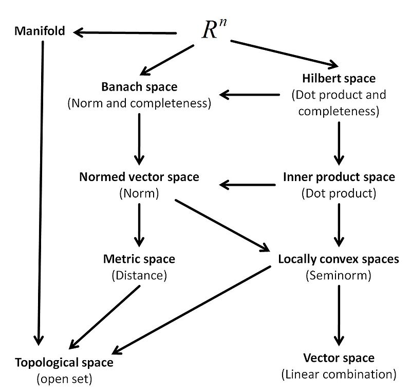
These included things like vector “fields” and topological vector spaces, of which metric spaces are a subset, of which normed vector spaces are a subset, of which inner product spaces and banach spaces are subsets, of which Hilbert spaces are a subset (etc). The latter, (particularly complex-valued Hilbert Spaces), are ubiquitous in quantum mechanics and quantum field theory for example. There may also come a point at which a student comes to learn that some vectors are also a subset of a class of mathematical objects known as “tensors.” Although not all vectors are tensors, all first order (or Rank 1) tensors are actually vectors, and although not all scalars are tensors, all zeroth order (or Rank 0) tensors are scalars.

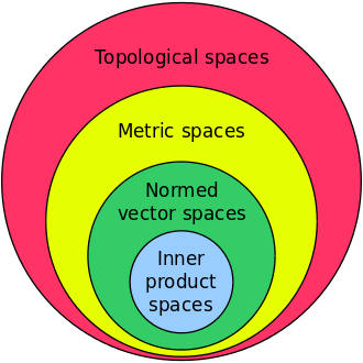
In actuality, the hierarchy is a bit more involved than depicted here, and understanding it would require covering some concepts such as “completeness” from a branch of math known as functional analysis, which I will not attempt to cover here.

Don’t worry about not knowing what distinguishes these types of spaces from one another right now. The point is to state up front that there multiple levels to this concept of vectors, instead of simply conveniently neglecting to mention that until it can’t be put off any longer, as is often done in the earlier University courses. So rather than getting lost down that rabbit hole, just know there are a few basic operations and notational conventions to understand for vectors in the sense of a “quantity possessing a magnitude and a direction,” but that those are but a special case of a broader and very useful mathematical concept that has applications in various scientific sub-disciplines.

If there is a high enough demand, I can go over vector multiplication (i.e. dot products/inner products and cross products), scalar projections, vector projections, vectors as functions of independent variables, vector calculus, the concept of a vector space, and various useful operations involving vectors and vector functions in subsequent posts.